One of the most important and functional items in Google Sheets is freezing a header row.
Freezing a header row will allow you to scroll through a large number of rows without having to scroll back to the top to check the row descriptions. Freezing a header row will also keep the header row from sorting into the rest of your data.
Freezing a header row will also help when setting a sorting filter.
Step One
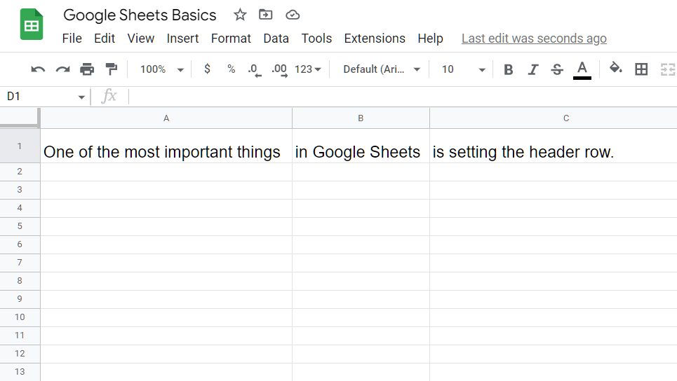
Find the header row. In this example, I have added text in columns A, B, and C of the first row. Depending on the data you are working with, this row may already exist. Generally, this row will include the description of the column’s data.

Step Two
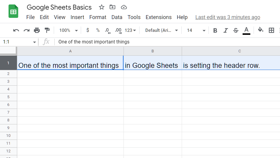
In order to select the row, click the number to the left of the row. In this example, the header information is in row 1.

Step Three
Find the header row. In this example, I have added text in columns A, B, and C of the first row. Depending on the data you are working with, this row may already exist. Generally, this row will include the description of the column’s data.

Step Four (Bonus Tip)
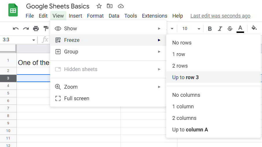
Clicking View and then Freeze usually only shows shows options for freezing one or two rows. But if you click any row, the menu will allow you to freeze up to any row you choose. This is especially beneficial if you are in need of space for company logos or other information above your header row.
